Investigating the relationship between PM 2.5 and Lead air measurements in California

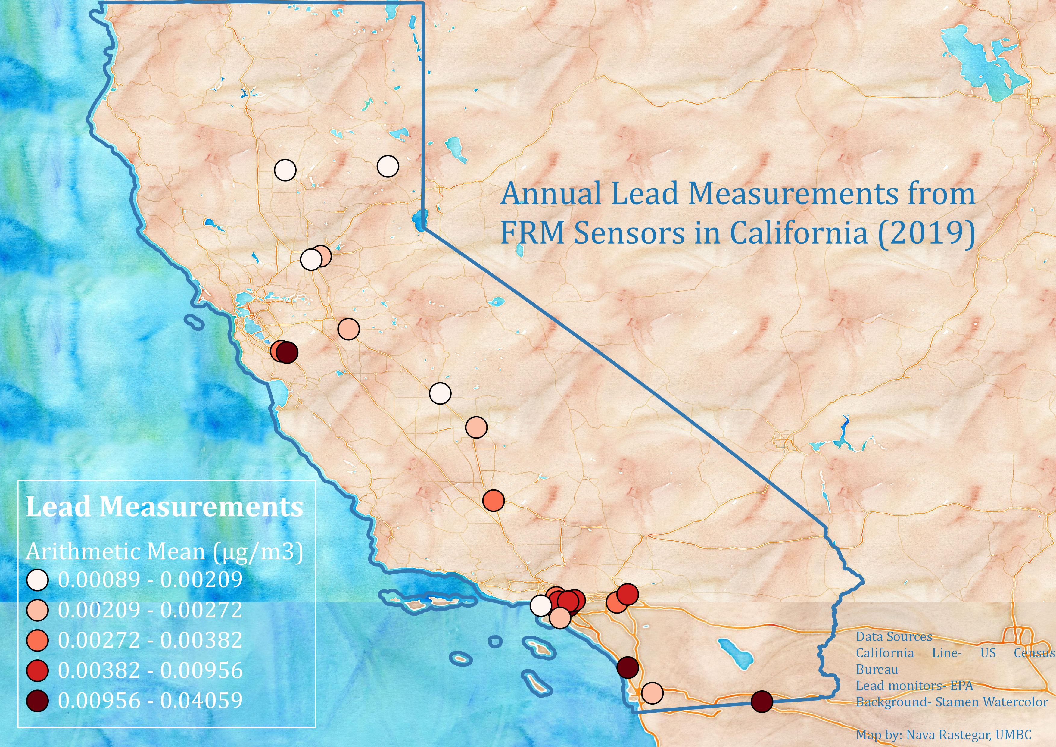
I downloaded 2019’s annual concentration by monitor from the EPA’s Air Data. I selected only the lead and PM 2.5 observations from California, and then further reduced the data by limiting points to only to the parameter measurements of PM 2.5 Local Conditions and Lead Local Conditions, to have comparable measurements, and only data where no ‘events’ were included (ie forest fires) to limit outliers. I then pared down the data so there was only one measurement of lead and one of PM 2.5 per point, by selecting only the machine with the most active measurement days per unique point. This left 103 points. Notably, there are about four times as many PM 2.5 monitors in this dataset as lead monitors.


Using QGIS, I created three buffers surrounding the lead monitors- one of 50 km, one of 10 km and one of 1 km. I created three files in which I performed a one-to-many spatial join between the PM 2.5 monitors and each of the Lead monitors in whose respective buffers they fell.


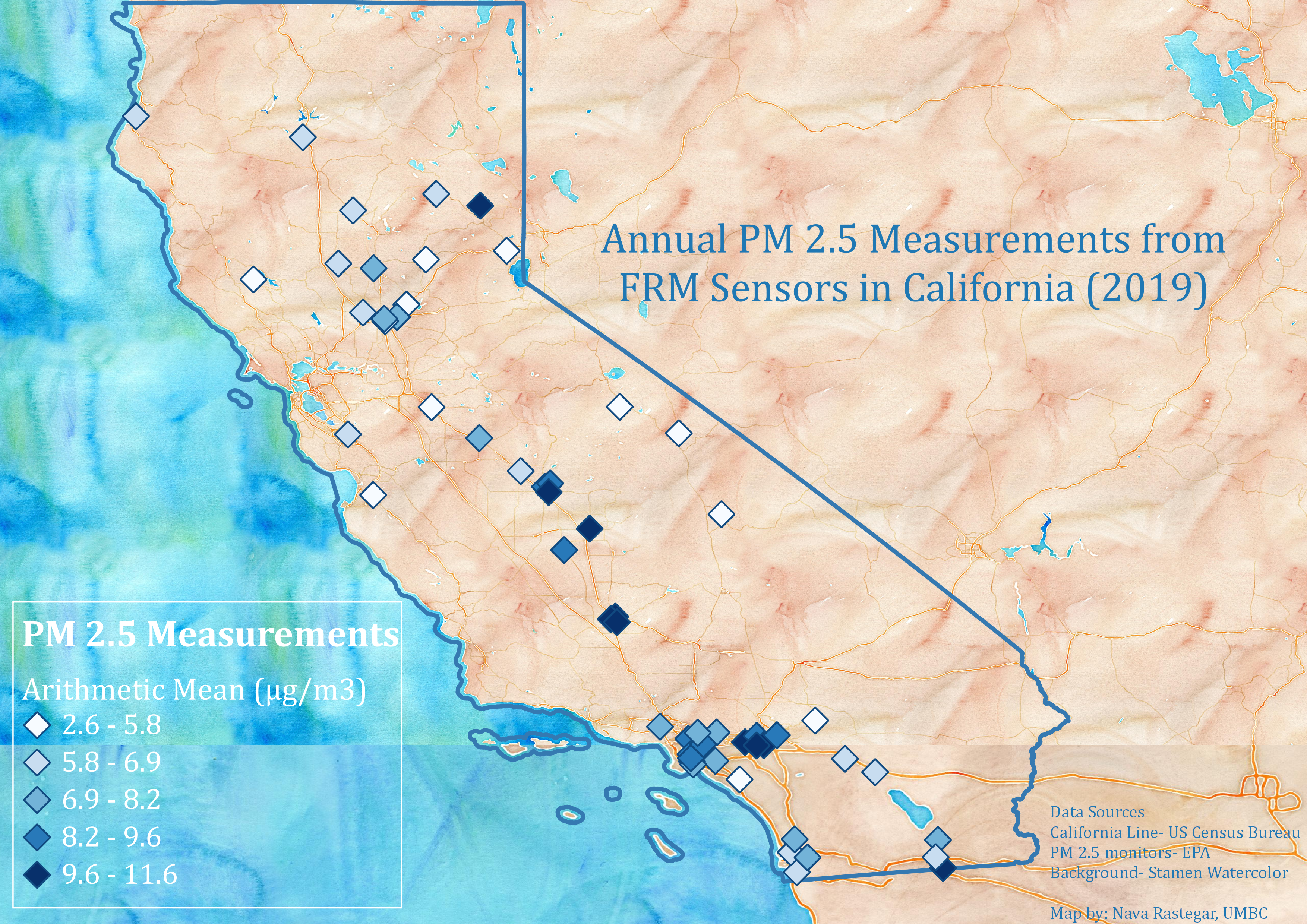
The dataset was exported into R, where I first performed a Moran’s I test on each parameter in order to determine whether there were significant clusters of high or low measurments. While the Moran’s I results for PM 2.5 measurements showed that there were signifcant clusters of high-high values (using alpha=.05), the test found no significant level of clustering of lead measurements.
I then created a linear model for each of the joined datasets, to determine if there was significant correlation between the arithmetic mean of lead measurements and the arithmetic mean of PM 2.5 measurements obtained near them. Unfortunately, none of the linear models showed any significant relationship between the measurements. Also, none had an R-squared above .2, indicating that the nearby PM 2.5 measurements explained little of the variation in Lead measurments. Even the 1km buffer join was well outside of the significance level (p> .1 as compared to alpha=.05), which is particularly disappointing as the 10km buffer was designed to only join the monitors located at the same site. This did not change even when data was transformed in order to decrease heteroskedasticity.

Next steps

Perhaps different combinations of comparable parameter types would reveal different relationships. A test including monitors across the US may also have different results. I would like to perform a test on a spatial error or spatial lag model as well, though I have had difficulty determining the best way to develop such tests on multiple point variables. Finally, a more complex but possibly more complete analysis would compare daily data rather than mean annual data, and take into account both time and space in determining a relationship.